The goal of carfollowingmodels is to make several car following models available in R for numerical simulation.
Installation
carfollowingmodelsis not on CRAN yet. But you can download the development version from GitHub with:
# install.packages("devtools")
devtools::install_github("durraniu/carfollowingmodels")
You need to have Rtools installed which you can download and setup using the instructions here.
Example
To use any car-following model, you need to provide the lead vehicle data, initial position, speed and/or acceleration of following vehicle(s), and model parameters.
The models used in this package are cited below:
| Model | Citation |
|---|---|
| Intelligent Driver Model | Treiber and Arne Kesting (2013) |
| Gipps Model | Gipps (1981) |
| Wiedemann 74 Model | Wiedemann and Reiter (1992); Higgs, Abbas, and Medina (2011) |
Following shows an example with 5 following vehicles. The lead vehicle is moving at 13.9 m/s at the reference position of 100 m.
# Time
last_time <- 3000 ## s
time_frame <- 0.1 ## s
Time <- seq(from = 0, to = last_time, by = time_frame)
time_length <- length(Time)


## Lead vehicle
vn1_first <- 13.9 ## first speed m/s
xn1_first <- 100 ## position of lead vehicle front center m
bn1_complete <- c(rep(0, 15000),
                  rep(0.05, 2000),
                  rep(-1, 3000),
                  rep(0, 8000),
                  rep(-5, 2001))


#############################################
### Complete speed trajectory of Lead vehicle
#############################################

vn1_complete <- rep(NA_real_, time_length) ### an empty vector
xn1_complete <- rep(NA_real_, time_length) ### an empty vector

vn1_complete[1] <- vn1_first
xn1_complete[1] <- xn1_first

for (t in 2:time_length) {

 ### Lead vehicle calculations
 vn1_complete[t] <- vn1_complete[t-1] + (bn1_complete[t-1] * time_frame)

 vn1_complete[t] <- ifelse(vn1_complete[t] < 0, 0, vn1_complete[t])


 xn1_complete[t] <- xn1_complete[t-1] + (vn1_complete[t-1] * time_frame) +
  (0.5 * bn1_complete[t-1] * (time_frame)^2)

}

## Lead vehicle data in a dataframe
ldf <- data.frame(Time, bn1_complete, xn1_complete, vn1_complete)
Intelligent Driver Model (IDM)
To predict the trajectories of the 5 following vehicles, you can use any car-following model available in this package. For example, the simulate_idm() function uses the Intelligent Driver Model as shown below. For more details on input arguments, type ?simulate_idmin the console.
library(carfollowingmodels)

## Run the IDM function:
results_idm <- simulate_idm(

resolution=0.1,
N=5,

dfn1=ldf,
xn1="xn1_complete",
vn1="vn1_complete",

xn_first=list(85, 70, 55, 40, 25),
vn_first=list(12, 12, 12, 12, 12),
ln=list(5, 5, 5, 5, 5),

a=2,
v_0=14.4,
small_delta=1,
s_0=4,
Tg=1,
b=1.5
)


head(results_idm)
#>   fvn Time    xn1  vn1 ln1         bn       xn       vn       sn    deltav
#> 1   1  0.0 100.00 13.9   5 -1.4407191 85.00000 12.00000 15.00000 -1.900000
#> 2   1  0.1 101.39 13.9   5 -1.1565350 86.19280 11.85593 15.19720 -2.044072
#> 3   1  0.2 102.78 13.9   5 -0.9399018 87.37261 11.74027 15.40739 -2.159725
#> 4   1  0.3 104.17 13.9   5 -0.7704464 88.54193 11.64628 15.62807 -2.253716
#> 5   1  0.4 105.56 13.9   5 -0.6351232 89.70271 11.56924 15.85729 -2.330760
#> 6   1  0.5 106.95 13.9   5 -0.5252076 90.85646 11.50573 16.09354 -2.394273
#>    sn_star
#> 1 9.418207
#> 2 8.860068
#> 3 8.420694
#> 4 8.069309
#> 5 7.785079
#> 6 7.553349
Now you can plot the results:
library(tidyverse)
#> Warning: package 'tidyverse' was built under R version 4.0.4
#> -- Attaching packages --------------------------------------- tidyverse 1.3.0 --
#> v ggplot2 3.3.3     v purrr   0.3.4
#> v tibble  3.1.1     v dplyr   1.0.5
#> v tidyr   1.1.3     v stringr 1.4.0
#> v readr   1.4.0     v forcats 0.5.1
#> Warning: package 'tibble' was built under R version 4.0.5
#> Warning: package 'tidyr' was built under R version 4.0.5
#> Warning: package 'dplyr' was built under R version 4.0.5
#> -- Conflicts ------------------------------------------ tidyverse_conflicts() --
#> x dplyr::filter() masks stats::filter()
#> x dplyr::lag()    masks stats::lag()

## Position
results_at_time_0_LV <- subset(results_idm, fvn==1 & Time ==0)
results_at_time_0_FV <- subset(results_idm, Time ==0)

ggplot() +
  geom_rect(data = results_at_time_0_LV,
            aes(xmin = xn1 - ln1,
                xmax = xn1,

                ymin = 0.628,
                ymax = 3.028)) +
  geom_rect(data = results_at_time_0_FV,
            aes(group = fvn,
                fill = as.factor(fvn),
                xmin = xn - 5,
                xmax = xn,

                ymin = 0.628,
                ymax = 3.028)) +
  geom_hline(yintercept = 3.6, linetype = "longdash") +
  coord_fixed(ratio=1) +
  theme(legend.title = element_blank())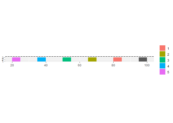
## Speed
ggplot(data = results_idm) +
  geom_line(aes(x = Time, y = vn, color = as.factor(fvn), group=fvn)) +
  geom_line(data = subset(results_idm, fvn==1),
            aes(x = Time, y = vn1, color = "LV Speed")) +
  theme(legend.title = element_blank())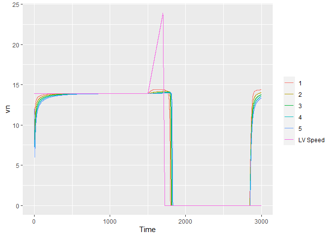
Gipps Model
results_gipps <- simulate_gipps(


resolution=0.1,
N=5,

dfn1=ldf,
xn1="xn1_complete",
vn1="vn1_complete",


xn_first=list(85, 70, 55, 40, 25),
vn_first=list(12, 12, 12, 12, 12),
ln=list(6.5, 6.5, 6.5, 6.5, 6.5),


an=2,
Vn=14.4,
tau=0.1,
bn=-1.5,
bcap=-2
)


head(results_gipps)
#>   fvn Time    xn1  vn1 ln1        bn       xn       vn       sn    deltav
#> 1   1  0.0 100.00 13.9 6.5 0.7815591 85.00000 12.00000 15.00000 -1.900000
#> 2   1  0.1 101.39 13.9 6.5 0.7585004 86.20391 12.07816 15.18609 -1.821844
#> 3   1  0.2 102.78 13.9 6.5 0.7359608 87.41552 12.15401 15.36448 -1.745994
#> 4   1  0.3 104.17 13.9 6.5 0.7139400 88.63460 12.22760 15.53540 -1.672398
#> 5   1  0.4 105.56 13.9 6.5 0.6924367 89.86093 12.29900 15.69907 -1.601004
#> 6   1  0.5 106.95 13.9 6.5 0.6714485 91.09429 12.36824 15.85571 -1.531760
#>      vn_ff    vn_cf
#> 1 12.00000 12.00000
#> 2 12.07816 12.83576
#> 3 12.15401 12.85679
#> 4 12.22760 12.87691
#> 5 12.29900 12.89615
#> 6 12.36824 12.91455


## Speed
ggplot(data = results_gipps) +
  geom_line(aes(x = Time, y = vn, color = as.factor(fvn), group=fvn)) +
  geom_line(data = subset(results_gipps, fvn==1),
            aes(x = Time, y = vn1, color = "LV Speed")) +
  theme(legend.title = element_blank())
#> Warning: Removed 60560 row(s) containing missing values (geom_path).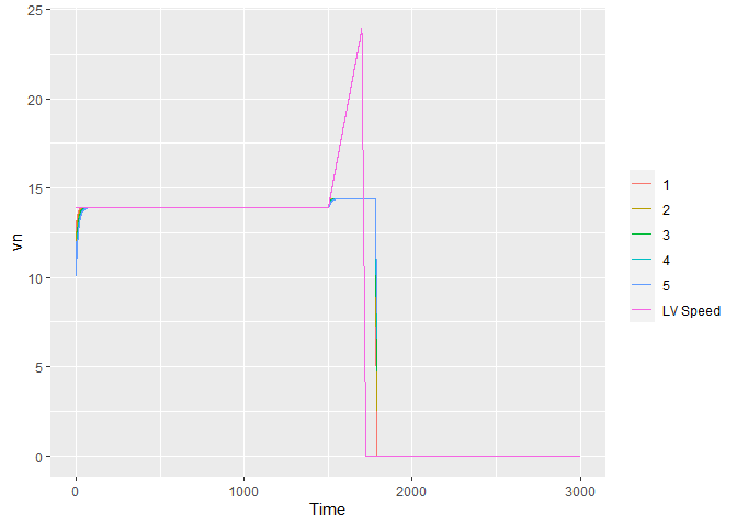
Wiedemann 74 Model (individual driver)
results_w74d <- simulate_wiedemann74_driver(
 resolution=0.1,
 N=5,
 dfn1=ldf,
 xn1="xn1_complete",
 vn1="vn1_complete",
 bn1="bn1_complete",
 xn_first=list(85, 70, 55, 40, 25),
 vn_first=list(12, 12, 12, 12, 12),
 ln=list(5, 5, 5, 5, 5),
 D_MAX=150,
 V_MAX=44,
 V_DESIRED=14.4,
 FAKTORVmult=0.001,
 BMAXmult=0.08,
 BNULLmult=0.25,
 BMIN=-5,
 CX=50,
 AXadd=2,
 BXadd=2,
 EXadd=2,
 OPDVadd=1.5
)


head(results_w74d)
#>   fvn Time    xn1  vn1 ln1        bn       xn       vn       sn    deltav AX
#> 1   1  0.0 100.00 13.9   5 0.5926839 85.00000 12.00000 15.00000 -1.900000  7
#> 2   1  0.1 101.39 13.9   5 0.5782258 86.20296 12.05927 15.18704 -1.840732  7
#> 3   1  0.2 102.78 13.9   5 0.5641204 87.41178 12.11709 15.36822 -1.782909  7
#> 4   1  0.3 104.17 13.9   5 0.5503591 88.62631 12.17350 15.54369 -1.726497  7
#> 5   1  0.4 105.56 13.9   5 0.5369335 89.84641 12.22854 15.71359 -1.671461  7
#> 6   1  0.5 106.95 13.9   5 0.5238353 91.07195 12.28223 15.87805 -1.617768  7
#>         BX      ABX CX      SDX        SDV      CLDV       OPDV      BMAX B_App
#> 1 6.928203 13.92820 50 20.85641 0.02560000 0.1024000 -0.1536000 0.5926839    NA
#> 2 6.945291 13.94529 50 20.89058 0.02681103 0.1072441 -0.1608662 0.5782258    NA
#> 3 6.961922 13.96192 50 20.92384 0.02801083 0.1120433 -0.1680650 0.5641204    NA
#> 4 6.978109 13.97811 50 20.95622 0.02919785 0.1167914 -0.1751871 0.5503591    NA
#> 5 6.993866 13.99387 50 20.98773 0.03037064 0.1214826 -0.1822238 0.5369335    NA
#> 6 7.009203 14.00920 50 21.01841 0.03152790 0.1261116 -0.1891674 0.5238353    NA
#>   B_Emg BNULL cf_state_sim
#> 1    NA  0.25 free_driving
#> 2    NA  0.25 free_driving
#> 3    NA  0.25 free_driving
#> 4    NA  0.25 free_driving
#> 5    NA  0.25 free_driving
#> 6    NA  0.25 free_driving


## Speed
ggplot(data = results_w74d) +
  geom_line(aes(x = Time, y = vn, color = as.factor(fvn), group=fvn)) +
  geom_line(data = subset(results_w74d, fvn==1),
            aes(x = Time, y = vn1, color = "LV Speed")) +
  theme(legend.title = element_blank())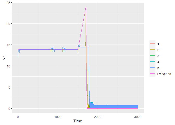
Outputs
| Variable | Description | Model |
|---|---|---|
| fvn | Following vehicle number | Common |
| Time | Time in seconds | Common |
| xn1 | Position of front center of the lead vehicle | Common |
| vn1 | Speed of the lead vehicle | Common |
| ln1 | Length of the lead vehicle | Common |
| bn | Acceleration (positive and negative) of the following vehicle | Common |
| xn | Position of front center of the following vehicle | Common |
| vn | Speed of the following vehicle | Common |
| sn | Spacing between the front bumper of the following vehicle and the front bumper of the lead vehicle (including the length of the lead vehicle) | Common |
| deltav | Speed difference (following vehicle speed - lead vehicle speed) | Common |
| sn_star | Desired spacing | IDM |
| vn_ff | Speed of following vehicle with free-flow equation | Gipps |
| vn_cf | Speed of following vehicle with car-following equation | |
| AX | Standstill spacing | Wiedemann74 |
| BX | Calibration Parameter | Wiedemann74 |
| ABX | Minimum following distance | Wiedemann74 |
| CX | Calibration Parameter | Wiedemann74 |
| SDX | Minimum following distance + drift due to unequal speed difference in opening and closing | Wiedemann74 |
| SDV | Speed difference when driver perceives approaching a slow lead vehicle | Wiedemann74 |
| CLDV | Speed difference when driver perceives closing in to lead vehicle | Wiedemann74 |
| OPDV | Speed difference when driver perceives losing lead vehicle | Wiedemann74 |
| BMAX | Acceleration in Free-driving | Wiedemann74 |
| B_App | Deceleration in Approaching | Wiedemann74 |
| B_Emg | Deceleration in Emergency-braking | Wiedemann74 |
| BNULL | Acceleration (positive and negative) in Following and at desired speed in Free-driving | Wiedemann74 |
| cf_state_sim | Driving state (Free-driving, Approaching, Following, Emergency-braking) | Wiedemann74 |
Compare Models
Comparing models is difficult as each model has at least a few unique parameters of its own. Nevertheless, following shows the speed of the fifth following vehicle as predicted by different models:
results_gipps_fv1 <- results_gipps %>%
  filter(fvn == 5)

results_idm_fv1 <- results_idm %>%
  filter(fvn == 5)

results_w74d_fv1 <- results_w74d %>%
  filter(fvn == 5)

ggplot() +
  geom_line(data = results_gipps_fv1 ,
            aes(x = Time, y = vn, color = "Gipps Speed")) +
  geom_line(data = results_idm_fv1 ,
            aes(x = Time, y = vn, color = "IDM Speed")) +
  geom_line(data = results_w74d_fv1 ,
            aes(x = Time, y = vn, color = "W74 Speed")) +
  geom_line(data = ldf ,
            aes(x = Time, y = vn1_complete, color = "LV Speed"), linetype = "longdash") +
  ggtitle("Speed")
#> Warning: Removed 12110 row(s) containing missing values (geom_path).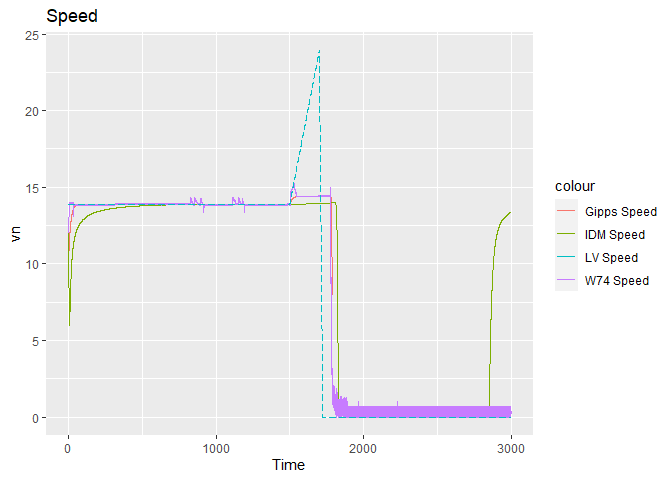
ggplot() +
  geom_line(data = results_gipps_fv1 ,
            aes(x = Time, y = sn, color = "Gipps")) +
  geom_line(data = results_idm_fv1 ,
            aes(x = Time, y = sn, color = "IDM")) +
  geom_line(data = results_w74d_fv1 ,
            aes(x = Time, y = sn, color = "W74")) +
  ggtitle("Spacing (including length of lead vehicle)")
#> Warning: Removed 12111 row(s) containing missing values (geom_path).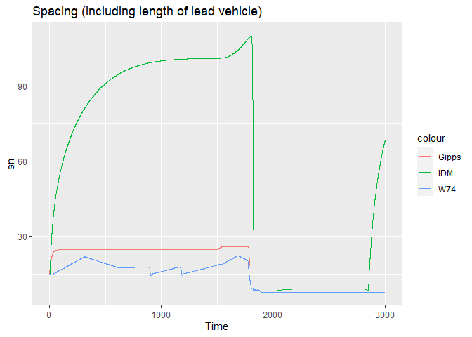
References
Gipps, P G. 1981. “A behavioural car following model for computer simulation.” Transportation Research Part B 15: 101–15.
Higgs, Bryan, MM Abbas, and Alejandra Medina. 2011. “Analysis of the Wiedemann Car Following Model over Different Speeds using Naturalistic Data.” 3rd International Conference on Road Safety and Simulation, 1–22.
Treiber, Martin, and Arne Kesting. 2013. “Traffic flow dynamics.” Traffic Flow Dynamics: Data, Models and Simulation, Springer-Verlag Berlin Heidelberg.
Wiedemann, Reiter, and U Reiter. 1992. “Microscopic traffic simulation: the simulation system MISSION, background and actual state.” Project ICARUS (V1052) Final Report. Brussels, CEC 2: 1–53.